STFT and CWT

0x10 基础
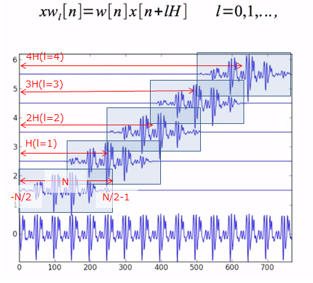
短时傅里叶变换(STFT)是对时变信号进行时频分析的一种方法,例如语音信号,可以得到局部时间的区域的频率和相位。短时傅里叶变换,顾名思义,也就是截断原信号为小段,对每段进行傅里叶变换。
数学公式是(来源:THE SHORT-TIME FOURIER TRANSFORM)
其中,
x(n) = n时刻的信号输入
w(n) = 窗函数 (例如汉明窗)
Xm(ω) = mR两侧加窗后信号的离散时间傅里叶变换DTFT
R = 前后的离散时间傅里叶变换DTFT的帧移距离
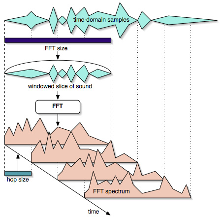
首先截取一段FFT长度的信号,和窗函数相乘后,对这一段短时间信号进行傅里叶变换得到周波数频谱。FFT点数决定了节点频率(frequency bin)的数量。
然后移动一个Hop Size再进行以上操作。Hop Size对应上式的帧移距离,一般至少需要在半个FFT点数以内,最好是四分一个FFT点数以内。
(来源:The Phase Vocoder – Part I)
另一个图例:
(来源:音楽アプリのための音声解析入門)
0x20 python代码实现
使用scipy库里面的fft和ifft以及窗函数,代码修改自Pythonで短時間フーリエ変換(STFT)と逆変換
# -*- coding: utf-8 -*-
# ==================================
#
#    Short Time Fourier Trasform
#
# ==================================
from scipy import ceil, complex64, float64, hamming, zeros
from scipy.fftpack import fft
from scipy import ifft
from scipy.io.wavfile import read

from matplotlib import pylab as plt


# ======
#  STFT
# ======
"""
x : 单声道输入x(n)
win : 窗函数w(n)
step : 频移R
"""
def stft(x, win, step):
    l = len(x) # 输入信号长度
    N = len(win) # 窗长度
    M = int(ceil(float(l - N + step) / step)) # 频谱图spectrogram的frame数,上面公式的m

    new_x = zeros(int(N + ((M - 1) * step)), dtype = float64)
    new_x[: l] = x # 如有必要,原信号适当延长,右边补零

    X = zeros([M, N], dtype = complex64) # spectrogram初始化, M行N列
    for m in range(M):
        start = step * m
        end = start + N
        X[m, :] = fft(new_x[start : end] * win)  # 每帧信号和窗函数相乘后,fft得出X的每行m的频率
    return X


# =======
#  iSTFT
# 恢复原信号
# =======
def istft(X, win, step):
    M, N = X.shape

    assert (len(win) == N), "FFT length and window length are different."

    l = (M - 1) * step + N     # 原信号长度
    x = zeros(l, dtype = float64)    # 初始化信号
    wsum = zeros(l, dtype = float64)

    for m in range(M):
        start = step * m
        end = start + N

        x[start : end] = x[start : end] + ifft(X[m, :]).real * win # 对X的每行进行ifft代入相应的时间
        wsum[start : end] += win ** 2  # 求窗函数的功率,得出归一化系数

    pos = (wsum != 0)
    x_pre = x.copy()

    x[pos] /= wsum[pos]  # 除以窗函数功率进行归一化
    return x
0x21 测试
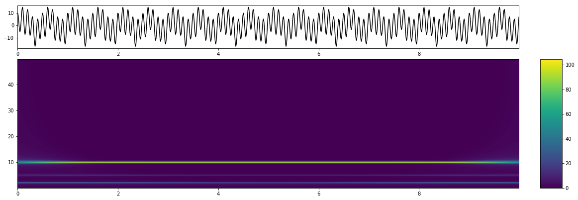
输入信号为 y= 5 sin(2 π 2 x) + 2 sin(2 π 5 x) + 10 cos(2 π 10 x)
信号由三个不同频率和幅度的正弦波组成。
import numpy as np

sampling_freq=100

x = np.arange(0, 10, 1/sampling_freq)
y = 5 * np.sin(2 * np.pi * 2 * x)  + 2 * np.sin(2 * np.pi * 5 * x)   + 10 * np.cos(2 * np.pi * 10 * x)
freq_max=int(sampling_freq/2)    # this is the maximum frequency detectable, according to the uncertainty principle 由采样定理可知
time_max=x.max()

fftLen = 512  # FFT点数
win = hamming(fftLen)  #汉明窗
step = fftLen // 4   # hop size选为1/4个FFT点数

### STFT
spectrogram = stft(y, win, step)

### iSTFT
resyn_data = istft(spectrogram, win, step)

### Plot
plt.rcParams['figure.figsize'] = (20, 12)
fig = plt.figure()
fig.add_subplot(311)
plt.plot(y)
plt.xlim([0, len(y)])
plt.title("Input signal", fontsize = 20)
fig.add_subplot(312)
plt.imshow(abs(spectrogram[:, : fftLen // 2 + 1].T), extent=[0, time_max, 0.1, freq_max], aspect = "auto", origin = "lower") # 这里选用numerical scale
plt.title("Spectrogram", fontsize = 20)
fig.add_subplot(313)
plt.plot(resyn_data)
plt.xlim([0, len(resyn_data)])
plt.title("Resynthesized signal", fontsize = 20)
plt.show()

0x30 对比—连续小波分析
原理略。
- 入门易懂的文章可以参考小波信号处理。
- 课程可以参考清华大学小波分析及其工程应用的课程pdf,可以下载
- 还有The Wavelet Tutorial
- The Illustrated Wavelet Transform Handbook
一般来说,对于瞬间突变信号,和多重解像度信号来说小波分析更加有优势。
python库有scipy.signal.cwt(),PyWavelets,mlpy和swan/PyCWT等。下面采用swan。
from swan import pycwt


omega0 = 8

freqs=np.arange(0.1,freq_max,0.25)  # be careful to choose the range of this freqs
r=pycwt.cwt_f(y,freqs,sampling_freq,pycwt.Morlet(omega0))   # morlet小波
rr=np.abs(r)

plt.rcParams['figure.figsize'] = (20, 6)
fig = plt.figure()
ax1 = fig.add_axes([0.1, 0.75, 0.7, 0.2])
ax2 = fig.add_axes([0.1, 0.1, 0.7, 0.60], sharex=ax1)
ax3 = fig.add_axes([0.83, 0.1, 0.03, 0.6])

ax1.plot(x, y, 'k')

#img = ax2.imshow(np.flipud(rr), extent=[0, 20, freqs[0], freqs[-1]],
#                 aspect='auto', interpolation='nearest')
img = ax2.imshow(np.flipud(rr), extent=[0, time_max, freqs[0], freqs[-1]],
                aspect='auto', interpolation='nearest')     # change the extent to fit the range

fig.colorbar(img, cax=ax3)

#colorbar(ticks=[0,30,60]).set_ticklabels(["0","30","60"]) this only sets the tick, not the range of the colorbar
# usage: fig.colorbar(img, cax=ax3,ticks=[0,30,60]).set_ticklabels(["0","30","60"])

plt.show()
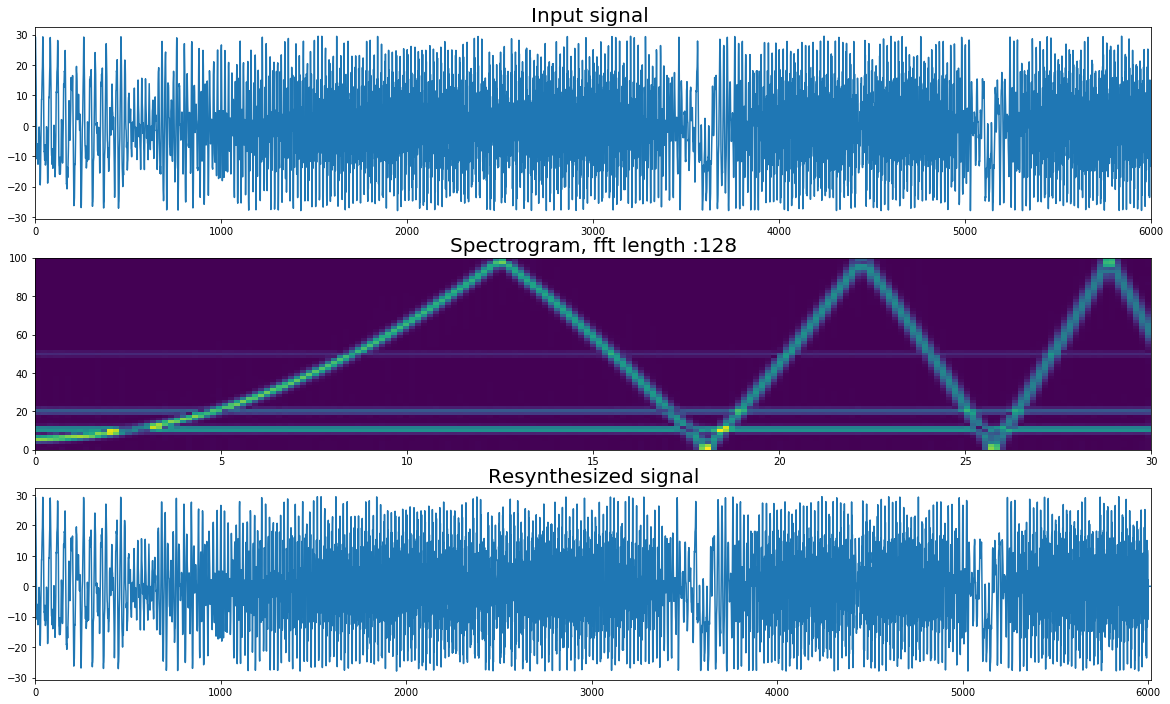
0x40 线性调频(Chirp)信号
为了对比,再加入一个线性调频信号
0x41 Chirp by STFT
# plus a quadratic chirp signal

from scipy.signal import chirp
sampling_freq=200


x2 = np.arange(0, 30, 1/sampling_freq)
y2 = 5 * np.sin(2 * np.pi * 20 * x2)  + 2 * np.sin(2 * np.pi * 50 * x2)   + 10 * np.cos(2 * np.pi * 10 * x2)   + 15 * chirp(x2, f0=5, f1=20, t1=5, method='quadratic')
freq_max=int(sampling_freq/2)    # this is the maximum frequency detectable, according to the uncertainty principle 由采样定理可知
time_max=x.max()

fftLen = 128
win = hamming(fftLen)
step = fftLen // 4

### STFT
spectrogram2 = stft(y2, win, step)

### iSTFT
resyn_data = istft(spectrogram2, win, step)

### Plot
plt.rcParams['figure.figsize'] = (20, 12)
fig = plt.figure()
fig.add_subplot(311)
plt.plot(y2)
plt.xlim([0, len(y2)])
plt.title("Input signal ", fontsize = 20)
fig.add_subplot(312)
plt.imshow(abs(spectrogram2[:, : fftLen // 2 + 1].T), extent=[0, time_max, 0.1, freq_max], aspect = "auto", origin = "lower")
plt.title("Spectrogram, fft length :"+ str(fftLen), fontsize = 20)
fig.add_subplot(313)
plt.plot(resyn_data)
plt.xlim([0, len(resyn_data)])
plt.title("Resynthesized signal", fontsize = 20)
plt.show()
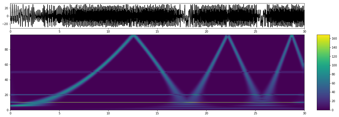
0x42 Chirp by CWT
from swan import pycwt

time_max=x2.max()


omega0 = 8

freqs=np.arange(0.1,freq_max,0.5)  # be careful to choose the range of this freqs
r=pycwt.cwt_f(y2,freqs,sampling_freq,pycwt.Morlet(omega0))
rr=np.abs(r)

plt.rcParams['figure.figsize'] = (20, 6)
fig = plt.figure()
ax1 = fig.add_axes([0.1, 0.75, 0.7, 0.2])
ax2 = fig.add_axes([0.1, 0.1, 0.7, 0.60], sharex=ax1)
ax3 = fig.add_axes([0.83, 0.1, 0.03, 0.6])

ax1.plot(x2, y2, 'k')


img = ax2.imshow(np.flipud(rr), extent=[0, time_max, freqs[0], freqs[-1]],
                aspect='auto', interpolation='nearest')     # change the extent to fit the range

fig.colorbar(img, cax=ax3)

#colorbar(ticks=[0,30,60]).set_ticklabels(["0","30","60"]) this only sets the tick, not the range of the colorbar
# usage: fig.colorbar(img, cax=ax3,ticks=[0,30,60]).set_ticklabels(["0","30","60"])

plt.show()
0x50 不确定性原理的制约
STFT在时域和频域的分解能力是受到海森堡不确定性原理约束的,窄窗(FFT点数少)的时间分辨率高而频率分辨率低,与此相反宽窗(FFT点数大)的时间分辨率低而频率分辨率高。


0x51 以STFT分析chirp做例子

动图能够看出不同长度的FFT点数对于得出的频谱分析图有影响
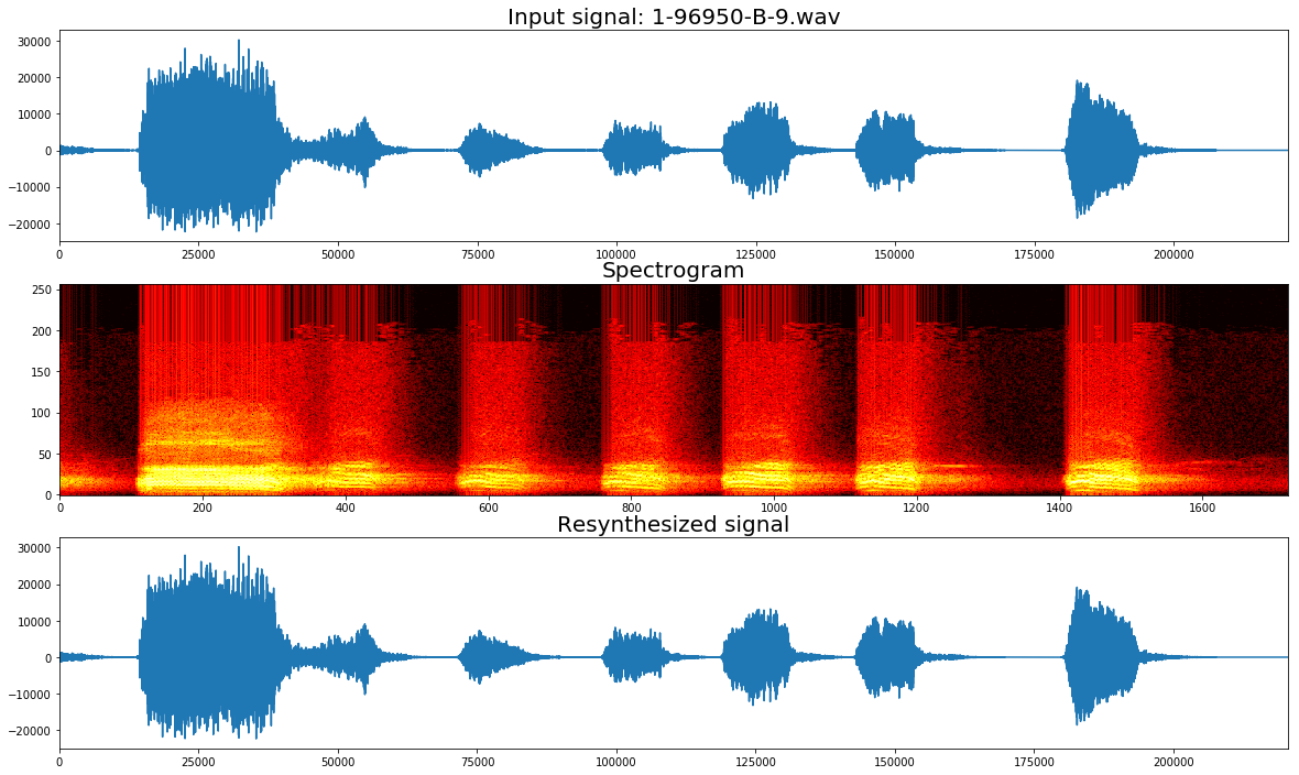
0x60 音频分析
ESC-50: Dataset for Environmental Sound Classification
使用环境音数据集里面的音频进行分析
0x61 STFT音频分析
wavfile = "1-96950-B-9.wav"
fs, data = read(wavfile)

data=data.astype(float64)  # change datatype


fftLen = 512
win = hamming(fftLen) # 汉明窗
step = fftLen // 4

### STFT
spectrogram = stft(data, win, step)

# for plot improvement
from scipy import histogram, log10
max_value = spectrogram.max()
spectrogram_dB= 20*log10(abs(stft(data, win, step)[:, : fftLen // 2 + 1]).T / float(max_value))


# adjust scale by removing data with low prob
hist, bin_edges = histogram(spectrogram_dB.flatten(), bins = 1000, normed = True)
hist /= float(hist.sum())
if True:  # false to turn off this
    rm_low = 0.1
    S = 0
    ii = 0
    while S < rm_low:
        S += hist[ii]
        ii += 1
    vmin = bin_edges[ii]
    vmax = spectrogram_dB.max()


### iSTFT
resyn_data = istft(spectrogram, win, step)


### Plot
plt.rcParams['figure.figsize'] = (20, 12)
fig = plt.figure()
fig.add_subplot(311)
plt.plot(data)
plt.xlim([0, len(data)])
plt.title("Input signal: "+wavfile, fontsize = 20)
fig.add_subplot(312)
#plt.imshow(abs(spectrogram[:, : fftLen // 2 + 1].T), aspect = "auto", origin = "lower")
plt.imshow(spectrogram_dB, origin = "lower", aspect = "auto", cmap = "hot", vmax = vmax, vmin = vmin)
plt.title("Spectrogram", fontsize = 20)
fig.add_subplot(313)
plt.plot(resyn_data)
plt.xlim([0, len(resyn_data)])
plt.title("Resynthesized signal", fontsize = 20)
plt.show()
出现错误信息,暂时不清楚原因,各位有idea的请指教
17: ComplexWarning: Casting complex values to real discards the imaginary part
21: VisibleDeprecationWarning: Passing `normed=True` on non-uniform bins has always been broken, and computes neither the probability density function nor the probability mass function. The result is only correct if the bins are uniform, when density=True will produce the same result anyway. The argument will be removed in a future version of numpy.
0x62 CWT音频分析
TBD
0x70 参考延伸
- THE SHORT-TIME FOURIER TRANSFORM)
- CLASSIC SPECTROGRAMS
- Short-time Fourier transform (Wikipedia)
- Pythonで短時間フーリエ変換(STFT)と逆変換
- Pythonで連続ウェーブレット変換(scipy, mlpy, swan)
- 小波信号处理
- 小波分析及其工程应用 - 清华大学
- The Wavelet Tutorial
- 能不能通俗的讲解下傅立叶分析和小波分析之间的关系?
- PyCWTで可視化の手続き
- PyCWT: spectral analysis using wavelets in Python
- https://github.com/kwinkunks/timefreak/blob/master/cwt.ipynb
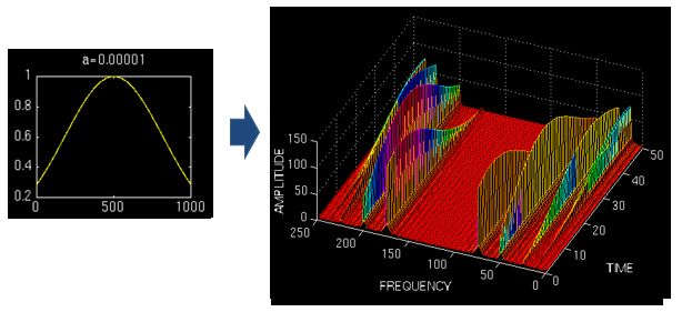
matlab版本:
վ HᴗP ի
This blog is under a CC BY-NC-SA 3.0 Unported License
Link to this article: https://hanspond.github.io/2018/09/18/STFT and CWT/